Recently, while working on a project, I had to verify that a set of data points was normally distributed. An easy, qualitative way to do this is to create a normal probability plot. The only problem was that I completely forgot how to do this, and all the explanations that I could find online sucked! So, here's a dead simple primer on normal probability plots, for boneheads like me with only basic statistics knowledge.
Let's say we have some dataset. In my case, it's the value of a pixel in an image over time. We can sort the elements of the dataset in ascending order, which allows us to assign each element a rank. In addition, let's also compute the z-score of each element.
| Value | Rank | z-score |
|---|---|---|
| 2062 | 1 | -4.76 |
| 2069 | 2 | -4.72 |
| 2122 | 3 | -4.43 |
| 2170 | 4 | -4.16 |
| 2216 | 5 | -4.01 |
| ... |
Now, here's the trick. We can use some math to determine the expected z-score of the nth element in a normally distributed dataset with the same size as ours. For example, we might say that the expected z-score of the 50th element in a sample of 100 normally distributed values is 0.
Using this, we can create a plot of our points where the x-axis is the expected z-score, and the y-axis is the actual z-score. If the distribution is really normal, the resulting points will fall on a straight line. Any deviations may tell you information about the true distribution, such as its skewness.
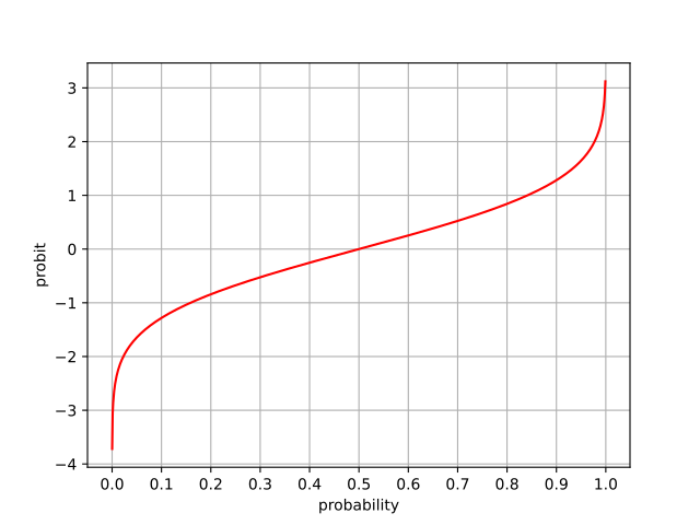
So how do we actually compute that expected z-score I just mentioned? Well, we can start with the normal CDF, which we'll write as . This function tells us the probability of a normally distributed random value being less than .
Notice that the CDF does the exact opposite of what we want. If we're considering the nth value of a set, we know the probability of a normal random variable being smaller than the point we're looking at, and want to know the z-score. Therefore, we should use the quantile function, which is the inverse of the CDF. For this reason, we'll write it as .
Now let's write a formula that converts rank and dataset size to z-score . We need to be careful since diverges at and . The following formula is used in many statistics packages:
Using this, we can assign our datapoints an expected z-score...
| Value | Rank | z-score | Expected z-score |
|---|---|---|---|
| 2062 | 1 | -4.76 | -2.97 |
| 2069 | 2 | -4.72 | -2.62 |
| 2122 | 3 | -4.43 | -2.44 |
| 2170 | 4 | -4.16 | -2.32 |
| 2216 | 5 | -4.01 | -2.23 |
| ... |
...and draw our normal probability plot:
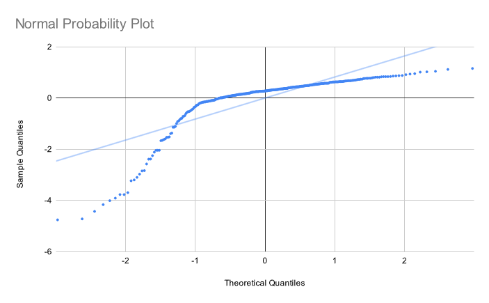
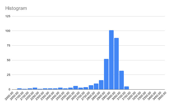
Oof. Not very normal at all. This is corroborated by the histogram:
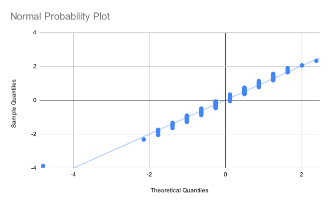
Let's try again, this time on a different set that is actually normally distributed. The normal probability plot:
and the histogram:
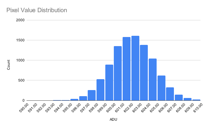
Nice! The probability plot looks a little weird due to quantization of the x-values, but this doesn't affect its functionality.
To learn more, I recommend checking out the section on the Normal Probability Plot from NIST's engineering statistics handbook.